Automated Machine Learning
• • ☕️☕️ 12 minute readSince the conception of the first electrical neurons in 1943 by neurophysiologist Warren McCulloch and mathematician Walter Pitts and the dawn of the first artificial neural network in the early 60’s, computer scientists wondered about how they could infer functions and distributions from input data from which they could generate accurate predictions. Given the sheer complexity of the task, Neural Nets were almost completely abandoned and underfunded in the AI Winter in favor of the more conventional Von-Neumann computer paradigms.

Automated Feature Engineering
Constructing features is a labor intensive task requiring technical know-how, data manipulation skills and a large amount of patience. Generating new predictors from existing ones is a tedious task and demands a lot of programming effort, yet it is so trivial. Automating this task spares the data scientist time that can be used on more important parts of the process loop. The creation and selection of new candidate features out of an existing pool of predictors the sole objective of automated feature engineering. But let us first take a step back and reflect on why we need feature engineering in the first place. Intuitively one could argue that the interaction between two predictors may lead to increased predictive power of the model. The feature selection can be explained by the classic garbage in garbage out principle.
- reduced overfitting
- reduced model complexity
- improved training times
- improved accuracy
Automated feature selection is basically aims to maximize a certain goal f.e. the model accuracy while minimizing the subset of features necessary to reach that goal. This can be realized with recursive selection procedures which account for feature collinearity and importance. If you want to learn more about feature engineering I recommend the following book:
Since this is a blogpost about the automation of feature engineering, I have a prior estimation that the feature engineering theory was already studied. Thus I skip ahead to the frameworks and explain quickly how we can realize it with simple code. There are not that many open-source choices out there (for now) but these are the top 3 frameworks I could conjure:
👉 https://www.featuretools.com/
👉 https://github.com/blue-yonder/tsfresh
👉 https://github.com/giantcroc/featuretoolsOnSpark
Featuretools is an incredibely useful library, saving me a lot of time for the remainder of my projects. The idea of featuretools is to first create an entityset, which are structured data tables with relationships, similar to database tables. The data input can come from a database, in-memory arrays, Excel sheets and other sources. The following entityset represents a classic business situation with customers, orders, areas, products and suppliers. Suppose we want to generate new features which could aid our model in predicting area-specific demand so that we can optimize our supply chain and/or stockpile:
Entityset: customers
  Entities:
    customers [Rows: 100, Columns: 5]
    orders [Rows: 3000, Columns: 9]
    areas [Rows: 12, Columns: 2]
    products [Rows: 10, Columns: 2]
    suppliers [Rows: 6, Columns: 3]
  Relationships:
    orders.customer_id -> customer.uuid
    orders.supplier_id -> suppliers.uuid
    clients.area_id -> areas.uuid
    orders.product_id -> products.uuid
Given this entityset we can now generate our new features simply by calling a method passing it the required aggregation and transformation primitives. We also can include a set of variables the generator has to ignore, or custom primitives which are manually put in. There is a whole list of primitives that can be used, so the data scientist just needs to focus on which ones best suit the problem.
features, feature_names = featuretools.dfs(
    entityset=es,
    target_entity='clients',
    agg_primitives=[
        'std', 'min', 'max', 'mean', 'count',
        'trend', 'n_most_common', 'time_since_last',
        'avg_time_between'
    ],
    trans_primitives=[
        'years', 'month', 'weekday', 'percentile',
        'latitude', 'longitude'
    ],
    ignore_variables={“products”: “releaseYear”},
    max_depth=1,
    n_jobs=-1,
    verbose=True)
This generates hundreds of new features that may lead to increased model performance.
More in-depth examples: https://www.featuretools.com/demos/.
However, this is only half of the story, since we still need to select a relevant subset. Featuretools supplies us with a basic remove_low_information_features method to remove features which consist of entirely NULLs or only have one class, etc.
More advanced selection procedures, supported by sklearn, include:
- GenericUnivariateSelect: Univariate selector with configurable strategy
- SelectPercentile: Select features according to a percentile of the scores
- SelectKBest: Select features with the k highest scores
- SelectFwe: Select the p-values corresponding to Family-wise error rate
- SelectFpr: Select the p-values below alpha based on a FPR test
- SelectFdr: Select the p-values for an estimated false discovery rate
- SelectFromModel: Meta-transformer based on importance weights
- RFE: Feature ranking with recursive feature elimination
- RFECV: Recursive feature elimination and cross-validated selection
- VarianceThreshold: Feature selector that removes all low-variance features
For smaller datasets the sklearn library should suffice.

Neural Architecture Search (NAS)
For neural network classifiers and regressors we may need to develop a model which suits our problem. Some problems are so popular (f.e. object recognition or recommender systems) existing architectures can be used of the shelf. For other problems however, we may need to come up with a custom defined one. Two general approaches currently dominate the landscape. The former is called Neural Architecture Search, which will be the subject of this section, the latter is called transfer learning.
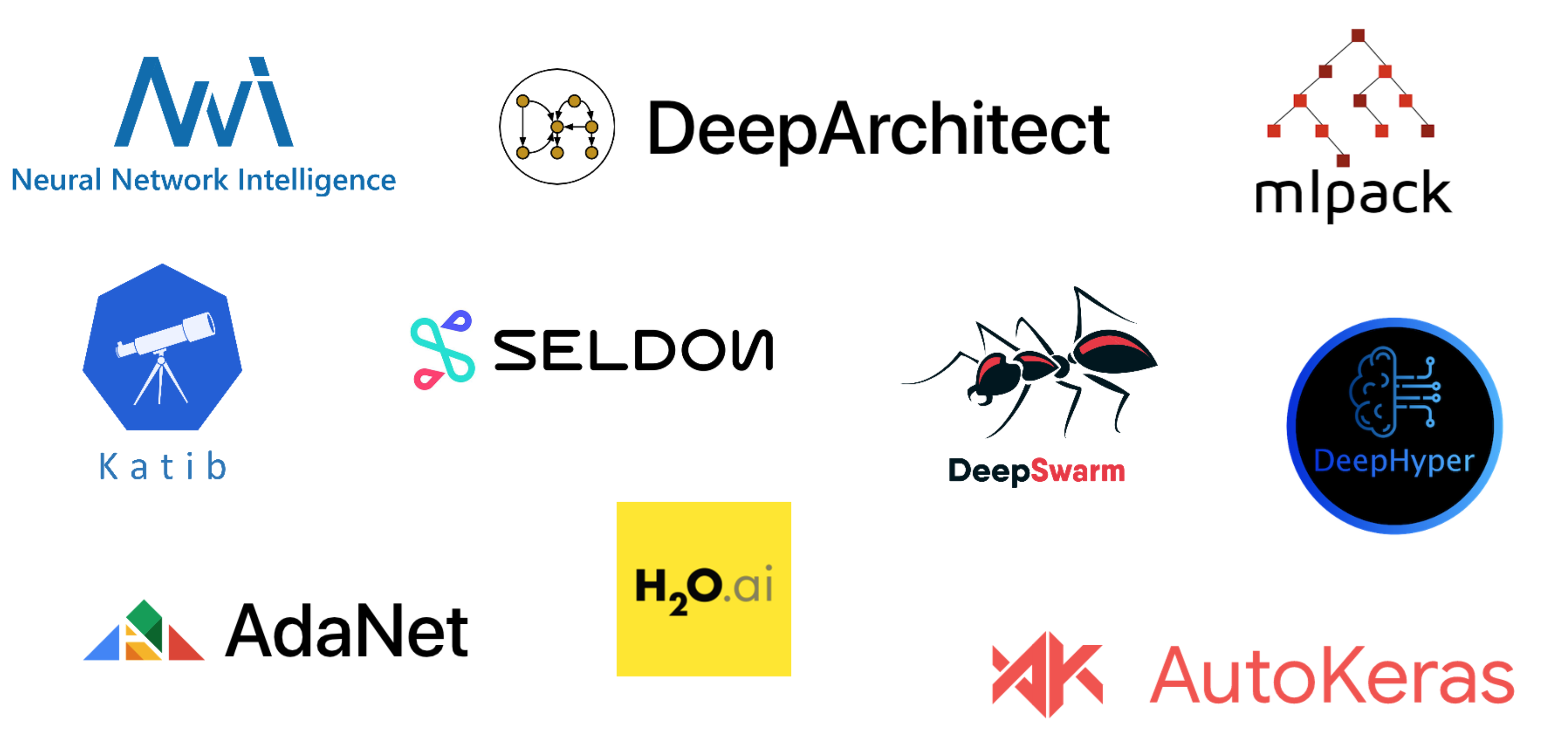
Neural Architecture Search is an optimization problem which in many cases is solved through the use of a metaheuristic, reinforcement learning or an autoregressive approach whereby new the search of new models is conditioned on already discovered ones. An example framework is DeepSwarm which generates models by the use of ant colony optimization. The architecture can change through widening (adding new neurons to an existing layer) or deepening (adding new layers). In april 2019, Google Research published MorphNet, which is the first major step towards efficient Neural Architecture Search.
MorphNet optimization mechanism are based on four main components:
- continuous relaxation (inducing sparsity)
- expansion (layer concatenation with shape compatibility constraints)
- iterative shrinking (low-weight edge removal)
- using the number of neurons as part of the loss function
Production-ready frameworks that can be used in an enterprise context are:
👉 AutoKeras (https://github.com/keras-team/autokeras)
👉 H2O (https://github.com/h2oai)
👉 NNI (https://github.com/microsoft/nni)
👉 MorphNet (https://github.com/google-research/morph-net)
With Neural Architecture Search, we can reduce our LOC down to a couple of lines. Take for example the classic MNIST benchmark on Autokeras:
from keras.datasets import mnist
from autokeras.image_supervised import ImageClassifier

# loading the MNIST dataset
(X_train, y_train), (X_test, y_test) = mnist.load_data()
X_train = X_train.reshape(X_train.shape + (1,))
X_test = X_test.reshape(X_test.shape + (1,))

# initialize the classifier
clf = ImageClassifier(verbose=True)

clf.fit(X_train, y_train, time_limit=30 * 60) #default time_limit = 24h
Initializing search.
Initialization finished.


╒==============================================╕
|               Training model 0               |
╘==============================================╛

Saving model.
+--------------------------------------------------------------------------+
|        Model ID        |          Loss          |      Metric Value      |
+--------------------------------------------------------------------------+
|           0            |   1.6572761310264468   |        0.98708         |
+--------------------------------------------------------------------------+


╒==============================================╕
|               Training model 1               |
╘==============================================╛

+--------------------------------------------------------------------------+
|    Father Model ID     |                 Added Operation                 |
+--------------------------------------------------------------------------+
|           0            |          ('to_conv_deeper_model', 9, 3)         |
+--------------------------------------------------------------------------+

Saving model.
+--------------------------------------------------------------------------+
|        Model ID        |          Loss          |      Metric Value      |
+--------------------------------------------------------------------------+
|           0            |   1.6572761310264468   |        0.98708         |
+--------------------------------------------------------------------------+
|           1            |   1.7632657293230296   |        0.98712         |
+--------------------------------------------------------------------------+

...

╒==============================================╕
|               Training model 7               |
╘==============================================╛

+--------------------------------------------------------------------------+
|    Father Model ID     |                 Added Operation                 |
+--------------------------------------------------------------------------+
|                        |          ('to_conv_deeper_model', 9, 3)         |
|                        |            ('to_wider_model', 14, 64)           |
|           2            |            ('to_wider_model', 9, 64)            |
|                        |          ('to_concat_skip_model', 1, 9)         |
|                        |           ('to_add_skip_model', 5, 9)           |
+--------------------------------------------------------------------------+

Saving model.
+--------------------------------------------------------------------------+
|        Model ID        |          Loss          |      Metric Value      |
+--------------------------------------------------------------------------+
|           0            |   1.6572761310264468   |        0.98708         |
+--------------------------------------------------------------------------+
|           1            |   1.7632657293230296   |        0.98712         |
+--------------------------------------------------------------------------+
|           2            |   1.6821355279535055   |        0.98804         |
+--------------------------------------------------------------------------+
|           3            |   1.751034566760063    |   0.9876400000000001   |
+--------------------------------------------------------------------------+
|           4            |   1.7889034859836102   |        0.98636         |
+--------------------------------------------------------------------------+
|           5            |   1.6054845724254847   |        0.98784         |
+--------------------------------------------------------------------------+
|           6            |   1.715640932880342    |   0.9876400000000001   |
+--------------------------------------------------------------------------+
|           7            |   1.6874338584020734   |   0.9872400000000001   |
+--------------------------------------------------------------------------+
Time is out.
As we can derive from the output, model 5 would be are goto model with an accuracy of 0.98784. However we could have aborted the search with an early stopping criterium since the accuracy of model 0 may already be satisfactory. Notice that we didn’t even had to define any layers!
Hyperparameter Grid Search
The final frontier of each AI scientist is discovering the right hyperparameters of the model. This is again a time consuming job which is nonetheless embarrassingly parallel. In order to exploit this characteristic we may need to call in the cavalry and opt for multithreading, multiprocessing or even functions as a service. Luckily there exist higher level frameworks which have developed solutions for this challenge. Production ready frameworks include:
👉 TPOT https://github.com/EpistasisLab/tpot
👉 Transmogrif https://transmogrif.ai/
👉 auto-sklearn https://automl.github.io/auto-sklearn/master/
👉 Hyperopt https://github.com/hyperopt/hyperopt
👉 Katib https://github.com/kubeflow/katib
Katib is my goto framework in a business context. As a cloud native practitioner I support the idea of running hyperparameter tuning on a Kubernetes cluster, it just seems like the perfect fit to me. Katib makes use of Kubeflow pipelines to distribute training jobs among the worker pool. An example configuration looks like:
apiVersion: "kubeflow.org/v1alpha3"
kind: Experiment
metadata:
  namespace: kubeflow
  name: pytorchjob-example
spec:
  parallelTrialCount: 3
  maxTrialCount: 12
  maxFailedTrialCount: 3
  objective:
    type: maximize
    goal: 0.99
    objectiveMetricName: accuracy
  algorithm:
    algorithmName: random
  trialTemplate:
    goTemplate:
        rawTemplate: |-
          apiVersion: "kubeflow.org/v1"
          kind: PyTorchJob
          metadata:
            name: {{.Trial}}
            namespace: {{.NameSpace}}
          spec:
           pytorchReplicaSpecs:
            Master:
              replicas: 1
              restartPolicy: OnFailure
              template:
                spec:
                  containers:
                    - name: pytorch
                      image: gcr.io/kubeflow-ci/pytorch-dist-mnist-test:v1.0
                      imagePullPolicy: Always
                      command:
                        - "python"
                        - "/var/mnist.py"
                        {{- with .HyperParameters}}
                        {{- range .}}
                        - "{{.Name}}={{.Value}}"
                        {{- end}}
                        {{- end}}
            Worker:
              replicas: 2
              restartPolicy: OnFailure
              template:
                spec:
                  containers:
                    - name: pytorch
                      image: gcr.io/kubeflow-ci/pytorch-dist-mnist-test:v1.0
                      imagePullPolicy: Always
                      command:
                        - "python"
                        - "/var/mnist.py"
                        {{- with .HyperParameters}}
                        {{- range .}}
                        - "{{.Name}}={{.Value}}"
                        {{- end}}
                        {{- end}}
  parameters:
    - name: --lr
      parameterType: double
      feasibleSpace:
        min: "0.01"
        max: "0.05"
    - name: --momentum
      parameterType: double
      feasibleSpace:
        min: "0.5"
        max: "0.9"
Kubernetes YAML files always seem overwhelming at first, but having such structured set-ups is exactly what a business might need. If you want to get started with Katib, you can find the Katib documentation here: https://www.kubeflow.org/docs/components/hyperparameter-tuning/overview/
Final remarks
This article was a high level overview of the 3 pillars of automated machine learning. For more in depth insights I recommend reading the academic literature which is listed at https://www.automl.org/automl/. The production ready frameworks are trending at the time of writing, but many new frameworks are on their way so the landscape may continue to evolve. A couple of lessons can be deducted from this article:
Overhyping AI may lead to over-inflated promises by developers and unnaturally high expectations of business leaders, which in turn may lead to the second fall of AI’s reputation.
Automated Machine Learning means resource intensive computations and asks for patience. So in terms of costs there will be a shift from R&D towards operations.
There is no single holy grail framework, experiment with different solutions and discover what works best for your problem.
NAS is not a certain path towards the perfect model, a group of AI engineers may come up with way more sophisticated models. One should regard this approach rather as a fast method to model prototyping.
Both feature engineering and hyperparameter tuning are incredibely useful and should be a mandatory part of the toolkit of a data scientist.
I hope you learned something new from reading this article, I’ll do my best to publish new articles in the near future.
