A theorethical overview of machine learning models
• • ☕️☕️☕️ 15 minute read
Analyzing data can be done in many ways. A common disclaimer is the so called No Free Lunch Theorem, which states that there is no single best model. Instead one should know how to use many models and choose what’s best depending on the data and our analytical goal. This article is a theorethic overview of the most common models used in machine learning practices today.
Predictive Analytics
In predictive analytics, the aim is to build an analytical model predicting a target measure of interest. The target is then typically used to tune the learning process during an optimization procedure. From another standpoint one can view predictive analytics as the problem of developing a model using historical data to make a prediction on new data where we do not have the answer. It can be described as the mathematical problem of approximating a mapping function (f) from input variables (X) to output variables (y). This is called the problem of function approximation.
Linear Regression
Regression predictive modeling is the task of approximating a mapping function (f) from input variables (X) to a continuous output variable (y). The most commonly used technique to model a continuous target variable is by using Linear Regression. A continuous target variable is a real-value, such as an integer or floating point value.
with
minimized by their sum of squares (often referred as Ordinary Least Squares = OLS). This technique is easy to understand/implement and thus contributes to operational efficiency. Other, more sophisticated techniques are ARIMA, VAR, GARCH and MARS.
Logistic Regression
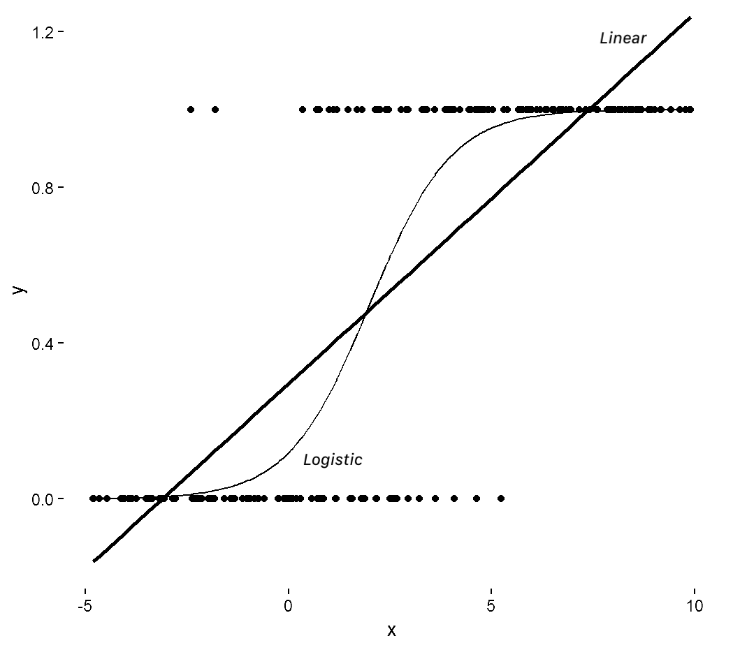
Do not get fooled by the regression term in its name. Logistic Regression is if not the most basic Machine Learning algorithm for binary-class classification.
When modeling the binary response target two problems arise:
- Errors are not normally distributed but follow a Bernoulli distribution.
- No guarantee that the target is between 0 and 1.
Therefore a bounding function was introduced:
so that
Interpretation: The amount of change required for doubling the primary outcome odds equals the so-called doubling amount:
To simplify the optimization, the logarithmic transformation of the likelihood function is taken and the corresponding logit can then be optimized using iteratively re-weighted least squares method.
Given this charachteristic we can use logistic regression to perform binary classification tasks in a time-efficient way. In practice it is often used to predict customer churn, advertisement efficiency, spam likelihood and much more.
Intermezzo: Variable Selection for Linear/Logistic Regression
Criterions for variable selection:
- More interpretable model
- More robust/stable model
- Reduced collinearity
- Operational efficiency
- Economic cost
- Regulations
| Model | Test Statistic |
|---|---|
| Linear Regression: | Student t-distribution with n-2 degrees of freedom. |
| Logistic Regression: | Chi-squared distribution with 1 degree of freedom |
For small numbers of variables, an exhaustive search can be used. Otherwise forward, backward or stepwise regression is preferred. Many ML toolkits such as sklearn have built-in search methods to perform variable selection.
Decision Trees
Decision trees are recursive partitioning algorithms. The calculations can be perfectly parallelized. The top root specifies the testing condition. The tree leaves assign the classifications. Implementations differ in the ways they answer the key decisions to build a tree, being:
- The splitting decision
- The stopping decision
- The assignment decision
Assignment Decision: typically just looks at the majority class.
Splitting Decision:
The splitting decision is based on the concept of impurity or chaos. Minimal impurity (= maximal purity) occurs when the variables are all of the same class. Maximal impurity is obtained when both classes represent 50% of the variables. Decision trees generally aim to minimize impurity in the data.
Quantitative Measures of Impurity
C4.5:
CART:
CHAID:
The weighted decrease in entropy thanks to the split is called the information gain:
It is clear that larger gains are preferred.
Stopping Decision:
Trees tend to overfit in the extreme case. In order to avoid this from happening, the dataset will be split into a training and validation set. A commonly used split is 70/30%. Where the validation set reaches its minimum, the procedure should be stopped. Decision trees can also be represented as sets of rules.
Whereas logistic regression estimates a linear decision boundary to separate the binary target variable. Decision trees model decision boundaries orthogonal to the axes.
Regression Trees
Decision trees can also be used to predict continuous targets. Impurity is measured by the Mean Squared Error, since a low MSE means less impurity.
Another way is to calculate the F-statistic. The assignment decision can be made by assigning the mean (or median) to each leaf node.
k Nearest Neighbors (kNN)
KNN algorithm is one of the simplest classification algorithm. Even with such simplicity, it can give good results. kNN can be used for both regression and classification tasks. It has a prior basis as it assumes that similar things exist in close proximity. In other words, similar things are near to each other. kNN uses the idea of similarity (also: distance, proximity, or closeness) which relates to calculating the distance between points on a graph based on a certain measuring fuction. Similar to recommender systems which predict your favorite products based on other user’s ratings, KNN operates by finding the distances between a target and all the examples in the data, selecting the specified number examples (K) closest to the target, then votes for the most frequent label (in the case of classification) or averages the labels (in the case of regression).
The algorithm is simple and easy to implement, as there’s no need to tune parameters (except for k), or make additional assumptions. The disadvantage is that it not scales well when naïvely implemented. However there exist optimizations:
Option I: Ball Trees
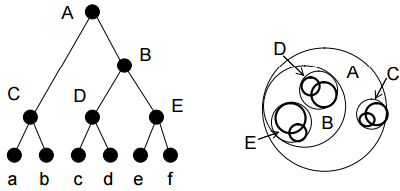
A Ball Tree is a special data structure that attempts to partition the training data in such a way that only a portion of the training data has to be searched. Ball Tree’s partition data into balls (hyperspheres). The efficiency of Ball Trees largely depends on the structure of the training data. If the training data can naturally be partitioned into circles/spheres/hyperspheres than the Ball Tree can be very efficient; however, data with no real structure(white noise) do not perform well. Data that is structured can possibly cause more paths to be pruned, while unstructured data may lead to more paths being explored. For this reason, the curse of dimensionality impacts Ball Trees heavily. As the dimensionality increase, it is less likely that the data can be partitioned into nice circles/spheres/hyperspheres. As more paths are explored the performance slowly begins to match brute force KNN.
Option II: KD Trees
A KD tree (= k-dimensional tree) is a space-partitioning data structure for organizing points in a k-dimensional space. KD trees are a useful data structure for several applications, such as searches involving a multidimensional search key (e.g. range searches and nearest neighbor searches). KD trees are a special case of binary space partitioning trees. The default setting of the kNN classifier in skLearn makes use of this optimization.
Support Vector Machines (SVM’s)
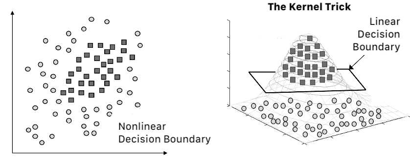
The bias of the support vector machine algorithm is that is tries to separate the data points with a maximal margin. When dealing with non-linear decision boundaries SVM’s rely on the kernel trick to create a linear decision boundary in a hyperplane based on a kernel method of choosing. SVM’s were often regarded as the best allround ML algorithms in town until the arrival of strong GPU’s and Deep Learning algorithms.
Neural Networks: Multi Layer Perceptrons
A Multi Layer Perceptron is a neural network with one input, one hidden and one output layer. The hidden layer essentially works like a feature extractor by combining multiple inputs into features. The hidden layer uses a non-linear transformation function, the output layer uses a linear one.
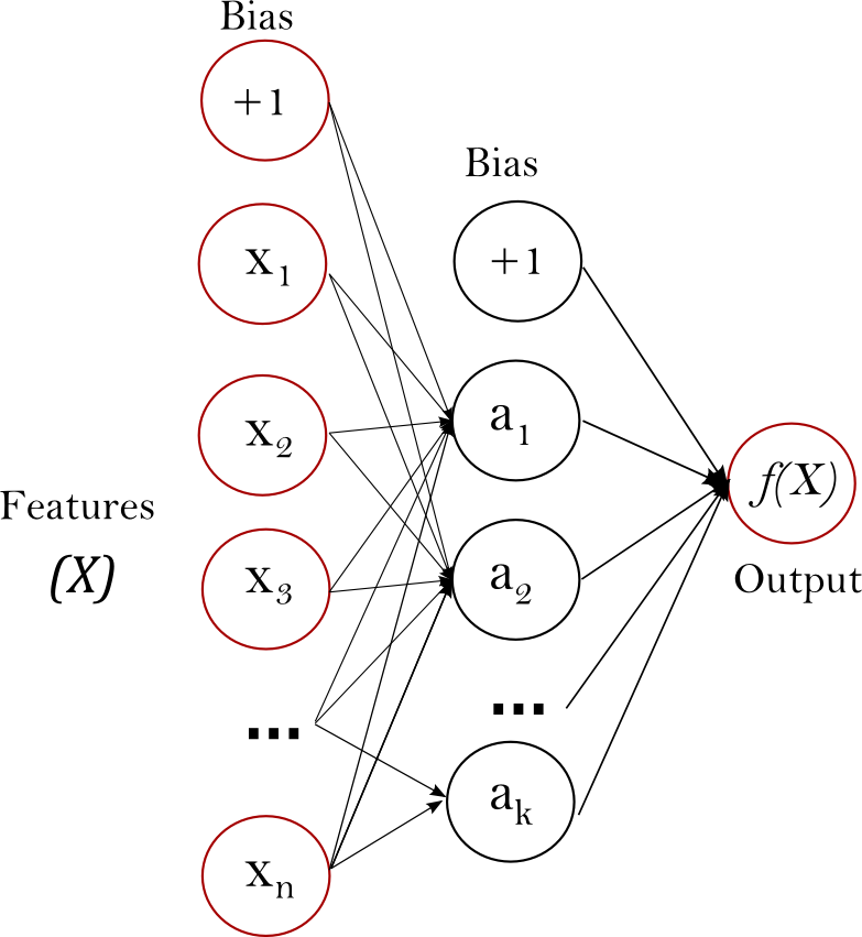
Activation functions:
- Logistic
- Hyperbolic
- ReLU
- Linear
Typically fixed for each layer. For classification it is common practice to adopt logistic transformation in the output layer, since the outputs can in that case be interpreted as probabilities. Neural networks with one hidden layer are universal approximators, capable of approximating any function to any degree of accuracy.
Hyperparameters:
For NN’s, the optimization is a lot more complex and the weights need to estimated using an iterative algorithm such as Gradient Descent or Levenberg-Marquardt. The cost function can have local minima, so iterative random weight initializations are necessary. Non-linear patterns require more hidden neurons.
Straightforward iterative algorithm:
- Split the data into a training, validation and test set.
- Vary the number of hidden neurons from 1 to 10 in steps of 1 or more.
- Train a neural network
- Measure its performance on the validation set
- Choose the optimal number of neurons
- Measure the performance on the independent test set
Hyperparameter tuning is truly a parallel problem and should therefore be optimized faster using techniques such as a fully-distributed grid search.
Neural Networks are so powerful that they can even model the noise in the training set, which should be avoided. To prevent overfitting, weight regularization closely related to Lasso regression implemented by adding a weight size term to the cost function of the neural network.
Neural networks with stacked hidden layers are often referred as deep learning models. They are extremely popular today because of the recent developments in GPU empowered analytics. Deep learning is a topic I will cover in detail in a future article.
Ensemble Methods
The aim of ensemble methods is to combine multiple (weak) predictive models into one more powerful model. Multiple models can cover different parts of the input space and as such complement each other’s deficiencies.
Bagging
Bagging (bootstrap aggregating) starts by taking B bootstraps from the underlying sample. A nice introduction to how bootstrapping works can be found here. Bootstrapping works provably works due to the law of large numbers and the convergence in probability. The underlying concepts are the empirical distribution function and plug-in principle.
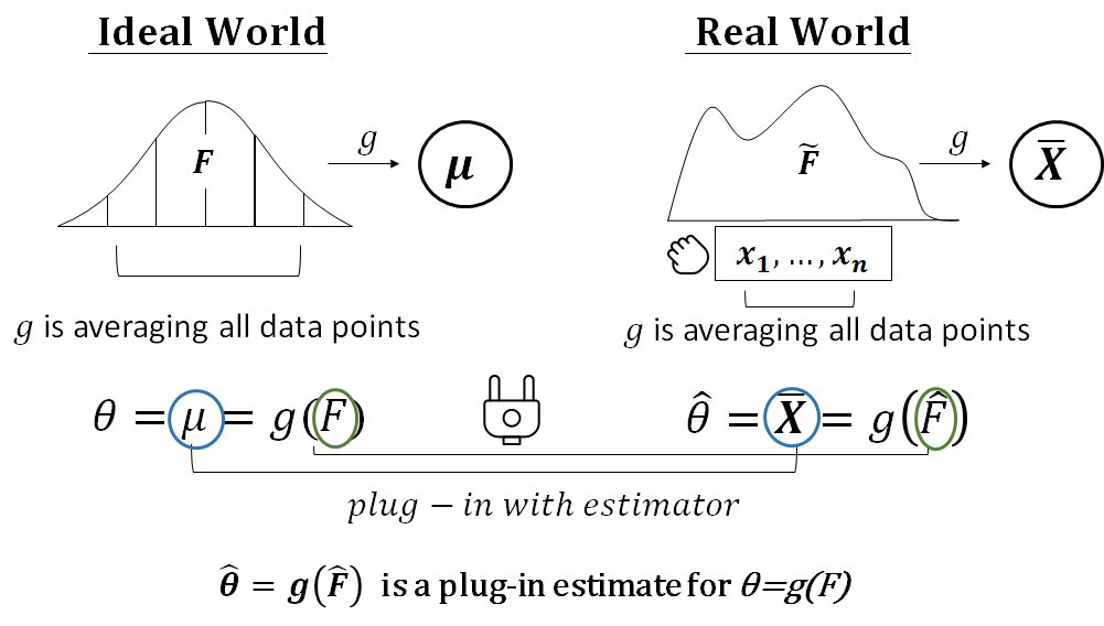
The idea is then to build a classifier (f.e. a decision trees, NN’s, linear regression) for every bootstrap. With classification tasks, major voting schemes are used. Whereas with regression tasks, the average outcome is taken.
If perturbing the dataset by means of bootstrapping can alter the model construct, bagging will improve overall accuracy. For models robust with respect to the underlying dataset, it will not give much added value. It generally reduces variance and can be used to avoid overfitting, therefore constructing a model that generalizes better.
Boosting
Boosting works by estimating multiple models using a weighted sample of the data. Although there is no single algorithm. Boosting techniques will often iteratively reweight the data according to the classification error whereby misclassified cases get more attention. The technique works with either directly weighted observations, or with a dataset sampling according to the weight distribution.
The final ensemble is then a weighted combination (strong learner) from all of the individual models (weak learners). Multiple loss functions may be used to calculate the error misclassification rate is the most popular.
Boosting algorithms can be based on convex or non-convex optimization algorithms. Convex algorithms, such as AdaBoost and LogitBoost, can be “defeated” by random noise such that they can’t learn basic and learnable combinations of weak hypotheses. Multiple authors demonstrated that boosting algorithms based on non-convex optimization, such as BrownBoost, can even learn from noisy datasets.
For binary classification, the general algorithm is as follows:
- Form a large set of simple features
- Initialize weights for training images
- FORALL training rounds:
- Normalize the weights
- FORALL features: train a classifier using a single feature and evaluate the training error
- Choose the classifier with the lowest error
- Update the weights of the training images: increase if classified wrongly by this classifier, decrease if correctly
- Form the final strong classifier as the linear combination of the T classifiers (coefficient larger if training error is small)
For multi-class classification:
The main flow of the algorithm is similar to the binary case. What is different is that a measure of the joint training error shall be defined in advance. During each iteration the algorithm chooses a classifier of a single feature (features that can be shared by more categories shall be encouraged). This can be done via converting multi-class classification into a binary one (a set of categories versus the rest), by introducing a penalty error from the categories that do not have the feature of the classifier.
A key advantage of Boosting is its simplicity. A potential drawback is that there may be risk of overfitting.
Random Forests
Random forests can be used with both classification and regression trees. Key in this approach is the dissimilarity amongst the base classifiers, which is obtained by adopting a bootstrapping procedure and the randomness of the splitting decisions.
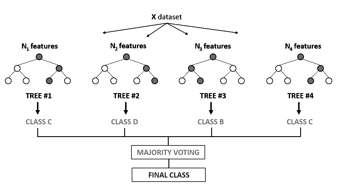
Diversity in base classifiers create an ensemble superior in performance. Random forests can be trivially implemented in the following way:
- Given a dataset with n observations and k inputs
- m = constant
- FOR t = 1 .. T
- Take a Boostrap sample of n observations
- Build a decision tree whereby for each node of the three randomly choose m variables on which to base the splitting decision
- Split on the best of this subset
- Full grow the tree without pruning
Descriptive Analytics
In descriptive analytics, often referred to as unsupervised learning, the aim is to describe patterns and features of our dataset.
Association Rules
An association rule is an implication of the form X => Y. The rules measure correlational associations and should not be interpreted in a causal way!
Support and confidence are two key measures to quantify strength of an association rule. A frequent item set is an item set for which the support surpasses a certain preset threshold. The confidence measures the strength of an association and is defined as the conditional probability of the rule consequent, given the rule antecedent.
The lift, also referred to as the interestingness measure, takes into account the prior probability of the rule consequent. A lift value (smaller) larger than 1 indicates a negative (positive) dependence or substitution (complementary) effect.
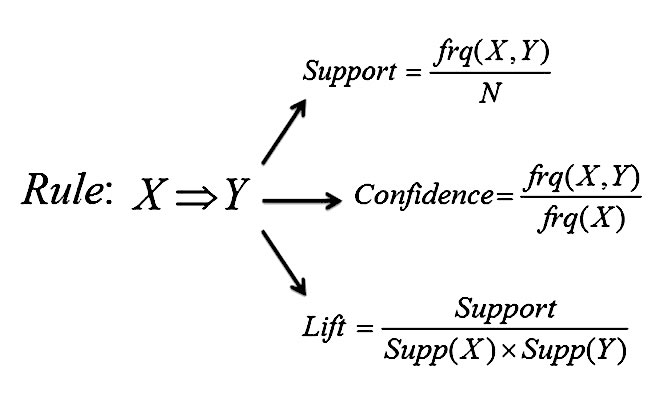
Post processing a rule miner entails:
- Filtering out trivial rules
- Performing sensitivity analysis
- Use appropriate visualisation facilities
- Measuring economic impact
Whereas association rules are concerned with what items appear together at the same time, sequence rules are concerned about what items appear at different times.
Clustering
The aim of clustering is to split up a set of observations into clusters such that the homogeneity within each cluster is maximized and the heterogeneity between clusters is also maximized. Techniques are either hierarchical (agglomerative or divisive) or non-hierarchical (k-means). In order to decide on the merger or splitting, a distance measure is needed. This is often Euclidian or Manhattan.
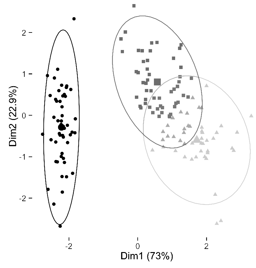
Various schemes are developed in order to define distance inbetween two clusters:
- Single Linkage
- Complete Linkage
- Average Linkage
- Centroid Method
Use a scree plot or dendogram to choose the optimal number of clusters.
Advantage: No prior number is specified
Disadvantage: Does not scale well
K-means clustering:
Select K observations as initial cluster centroids
Assign each observation to the cluster that has the closest centroid
When all observations are assigned, recalculate the position of the k centroids
Repeat until the centroid positions are stable
Self Organizing Maps:
Allows users to visualize and cluster high-dimensional data on a low-dimensional (rectangular/hexagonal grid) of neurons. A SOM is a feedforward neural network with two layers, whereby the output layer represents the grid. Each input is connected to all outputs. Beware to standardize the data to zero mean and unit derivation first! The neuron that is the most similar to a certain position is called the best matching unit.

Closing note
We overviewed different regression and classification methods such as Logistic Regression, SVM’s, Decision Trees, kNN and MLP’s. There is a lot to say about these algorithms still, there is a lot to say about other undiscussed algorithms as well, such as Bayesian Networks, Deep Learning and Graph Summarization techniques. In order to go more in depth, we will, in future articles, delve deeper in each of these algorithms by the use of practical code examples. For now I hope you enjoyed the summary of some of the most common used models one could use to conduct analytical exercise. A recommended book (I also have read) when interested:
